
In this blog series, I am exploring a few of my favourite algorithms in mathematics.
Last week, we looked at an algorithm that allowed us to convert a fraction into a continued fraction. This week, I want to focus on a more visual algorithm. Suppose you need to get someplace fast. What is the fastest route? These days, any smartphone can quickly calculate such a route for you. But how does your phone know? Is there some method, or does Google use magic?
The problem with finding the fastest route is that you cannot just pick the fastest road at each step. You must step back and consider all your options before settling on a course. Let me illustrate.

Imagine you are sitting at point A and need to travel to point D. It might be tempting to travel A -> B. Tempting, because 3 is less than 5, and you want to take the shortest path. However, if you do this, you will be stuck taking the road from B to D, which will make for a total of 7.
If instead, you travel A -> C -> D, you get a lower total of 6. Notice that you had to make the tough choice of starting with A -> C which was worth 5. This initially seems like a bad idea. But once you got going, you realized that the second part C -> D was only 1, a very short path. This more than made up for the pain of sitting and waiting so long in the first section.
Obviously, it isn’t too challenging to find the shortest path in the above example. There aren’t that many options. But in the real world, we have so many different paths to choose from. And ‘looking at all your options’ can be very overwhelming. Consider a slightly larger map:
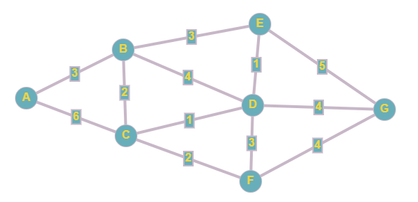
Now maybe you are great with directions and you can easily find your way to the shortest path from A to G. But looking at this huge mess of numbers makes my brain hurt. Thankfully, in 1959, Edsger Dijkstra discovered an algorithm for finding the shortest path.[1]
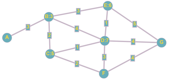
First begin with node A and label the adjacent nodes with the distance to each:

Select the next node (in this case B:3) and label all the connected nodes. For node E, we would label it 6, because 3 + 3 = 6. For node D, we would label it 7, because 3 + 4 = 7.
If a node (like node C) is already labeled, you have 2 choices
If the current number is smaller then delete the path and leave the current label
If the new path is shorter then delete the old path and use the new label
In the case of C, we would delete the useless 6 path connecting A and C, and update the label to 5, because 3 + 2 = 5
Keep repeating until you find the shortest path. So we would repeat our process with node C:

Repeat again with node E:

Repeat with node D:
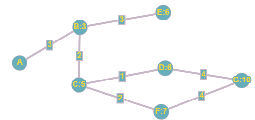
And one last time with node F:

Tada! We have found the shortest path from A to G, the length is 10 and you get there by travelling A -> B -> C-> D -> G. If we look back at our original graph, we can see just how far we have come in applying Dijkstra’s algorithm.


Pingback: Kruskal’s Algorithm | the Math behind the Magic