Juniper Green

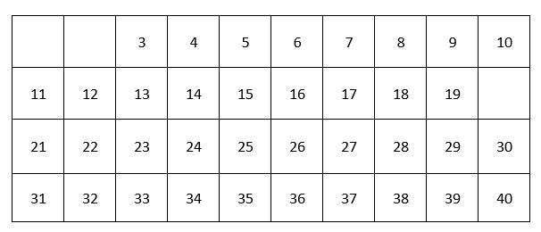
Today I want to investigate a mathematical game called Juniper Green. To play Juniper Green, you first begin with a grid of the numbers 1 through 40. Each player takes turns removing numbers from the grid. But they can’t pick just any number. Each number chosen must either be a factor or multiple of the previous player’s choice. If a player is unable to choose a number, then the game is over and they lose. Oh, and the person who goes first must pick an even number to start.

Let’s play. Suppose the first player chooses 20. The second player can now choose either a factor (1, 2, 5, 10) or a multiple (40):

Say they choose 2. Now the next player can choose either a factor (1) or a multiple (4, 6, 8, 10, etc.)

As the game progresses, it will become clear that choosing the number 1 is a very bad move. If someone takes the number 1, then their opponent can take any other number:

And there are some special numbers, prime numbers, that are particularly useful in Juniper Green. If a player takes 37, the game is over. There are no multiples of 37 in sight, the only factor of 37 is 1, and that number is gone.

If you play a few rounds of Juniper Green, it can feel pretty random. Sometimes you win, and sometimes you lose. Sure, there is some strategy, like not picking the number 1, but it also feels like luck plays a major role in this game.

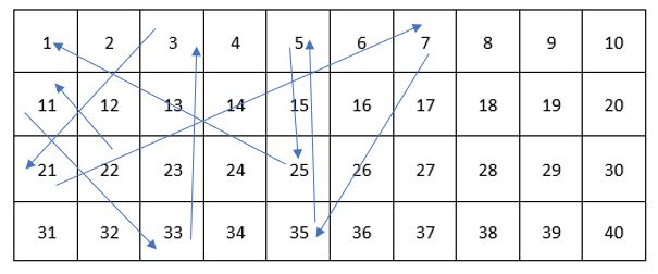
Believe it or not, the first player has a winning strategy. Consider the following sequence of moves, I will be player one and you will be player two. I start with 22. Next, there are only 2 possible options, either 2 or 11, and we will examine them individually.

Suppose you take 11. Next, I take 33. Because 33 is a large number, there are no multiples for you to take, you must take a factor. However, the only factor left is 3, so you must take 3.

Next, I take 21. Because 21 is a large number, there are no multiples for you to take, you must take a factor. However, the only factor left is 7, so you must take 7.

Next, I take 35. Because 35 is a large number, there are no multiples for you to take, you must take a factor. However, the only factor left is 5, so you must take 5.

Next, I take 25. Because 25 is a large number, there are no multiples for you to take, you must take a factor. However, the only factor left is 1, so you must take the number 1 and you lose.

To complete my victory, I take the prime number 37 and I win.

Now consider the other option, suppose you take the 2. Next, I take 26. Because 26 is a large number, there are no multiples for you to take, you must take a factor. However, the only factor left is 13, so you must take 13.

Next, I take 39. Because 39 is a large number, there are no multiples for you to take, you must take a factor. However, the only factor left is 3, so you must take 3.

Next, I take 21. Because 21 is a large number, there are no multiples for you to take, you must take a factor. However, the only factor left is 7, so you must take 7.

Next, I take 35. Because 35 is a large number, there are no multiples for you to take, you must take a factor. However, the only factor left is 5, so you must take 5.

Next, I take 25. Because 25 is a large number, there are no multiples for you to take, you must take a factor. However, the only factor left is 1, so you must take the number 1 and you lose.

To complete my victory, I take the prime number 37 and I win.

In either case, you lose. And your moves are tightly constrained. At each step, you only have one number you can pick. When you play against someone who knows this strategy, your doom feels inevitable. They have outmaneuvered you at every turn.

However, you can still have fun with this game, you just need to add more numbers! If you allow numbers 1 to 100, this strategy breaks down. If I start with 22, there are many possible moves other than 2 and 11. You could take a multiple, like 44, 66, or even 88! I wonder, is there a way to win at this new, expanded game of Juniper Green? Give it a try!

Alright, hopefully you gave the 1 to 100 version of Juniper Green a try. If you did, you might have realized that there is also a winning sequence in this version.

I start with 58. Next, there are only 2 possible options, either 2 or 29, and we will examine them individually.

Suppose you take 2. Next, I take 62. Because 62 is a large number, there are no multiples for you to take, you must take a factor. However, the only factor left is 31, so you must take 31.

I take 93, you must take 3.

I take 57, you must take 19.

I take 95, you must take 5.

I take 65, you must take 13.

I take 91, you must take 7.

I take 77, you must take 11.

I take 55, and since the 5 has already been removed, you must take the 1 and you lose.

To complete my victory, I can take the prime number 97 and I win.

Suppose you take 29. Next, I take 87. Because 87 is a large number, there are no multiples for you to take, you must take a factor. However, the only factor left is 3, so you must take 3. From here, the moves are the same as above.

I take 93, you must take 3.

I take 57, you must take 19.

I take 95, you must take 5.

I take 65, you must take 13.

I take 91, you must take 7.

I take 77, you must take 11.

I take 55, and since the 5 has already been removed, you must take the 1 and you lose.

To complete my victory, I can take the prime number 97 and I win.

The key to my victory is that I always picked a number too large for you to take multiples. Additionally, the number I picked only had one prime factor left on the board. By picking numbers in this way, I left you with no options. Your moves were always forced, and I was able to keep you dancing around the board until you had to take the number 1. Does this strategy work for the numbers 1 to 1000? What about 1 to 10000? Leave your answer in the comments below.

Kruskal’s Algorithm

In this blog series, I am exploring a few of my favourite algorithms in mathematics.

Last week, we looked at an algorithm that allowed us to find the fastest route between two points. Today, I want to discuss an algorithm for creating a network of roads. Suppose you work in infrastructure and you have been tasked with connecting a series of small towns. These towns are all isolated and it is your job to build roads to connect them.

One solution would be to build a bunch of roads until all the towns ‘feel connected.’ Perhaps something like this:

The obvious downside to this method is the cost. Each road costs money, and some of the roads are redundant. For example, consider the road from G to F. Sure, it would be nice for the residents of G to drive straight to F. However, we could save some money by removing that road, and residents could still get to F by first travelling through I:

Using the same reasoning, we could perhaps remove the road from G to H, since residents could travel G -> I -> H:

Taking this approach to its logical conclusion, we would like to design a road system that doesn’t have any ‘extra’ connections. In other words, each town is connected in some way to every other town, but there is only one route between them. A road system like this:

Success! Observe how each town is connected to every other town, and there are no extra roads. However, our haphazard approach to the problem has left the residents in town A and with a very long commute to town J. Even though A and J close together on the map, the route to travel from A to J is very long: A -> D -> C -> B -> H -> I -> J. If you built this road system, your office should be ready to deal with some angry phone calls! There must be a better way.

Enter Kruskal’s algorithm. In 1956, Joseph Kruskal discovered a method to link all these towns in the most
efficient way possible [1]. His method assigns a cost to all possible roads. In our case, we will estimate the cost to be the length of the road:

We will now use this expensive road system to help create a cheaper alternative as follows:

• Select the shortest road
  • If the addition of this road would form a loop, discard it
  • Otherwise, include it
• Repeat until all towns are connected

The shortest road on our map is between A and J with a value of 4. So we begin our construction with this single road.

Next, we will add the road between I and J with a value of 5, the road between B and J with a value of 7, and both roads H to I and G to I with a value of 8:

However, we are not able to add the road from A to B with a value of 9. If we were to connect A and B, that would create a loop: A -> B -> J -> A. While this extra road would be nice for the residents in town A, it is unnecessary, since they can just travel through town J to get to town B:

So we have to look elsewhere for another road to add to our growing network. Indeed, the road from H to I with a value of 10 works well.

All of the roads with a value of 11 are also ineligible for our road system because they also would create unnecessary loops.

However, we can add the roads of 12 and 16:

Success! Every town is connected and we have completed our network. Comparing this road system to our previous system shows how much progress we have made in eliminating redundant roads:

However, this elimination has come at a social cost. While our road system does connect every town, it does so in a brutally efficient manner. I suspect town C and D would not be very appreciative of how a simple road of length 19 between their neighbouring towns was slashed in the service of efficiency. Due to your mathematically-minded approach, they must travel a distance of 13 + 4 + 5 + 8 + 12 + 16 = 58 to visit with one another. This algorithm helps illustrate the fundamental problem in mathematics and in life; you can’t have your cake and eat it too.

---

[1] https://en.wikipedia.org/wiki/Kruskal%27s_algorithm

Shortest Path Algorithm

In this blog series, I am exploring a few of my favourite algorithms in mathematics.

Last week, we looked at an algorithm that allowed us to convert a fraction into a continued fraction. This week, I want to focus on a more visual algorithm. Suppose you need to get someplace fast. What is the fastest route? These days, any smartphone can quickly calculate such a route for you. But how does your phone know? Is there some method, or does Google use magic?

The problem with finding the fastest route is that you cannot just pick the fastest road at each step. You must step back and consider all your options before settling on a course. Let me illustrate.

Imagine you are sitting at point A and need to travel to point D. It might be tempting to travel A -> B. Tempting, because 3 is less than 5, and you want to take the shortest path. However, if you do this, you will be stuck taking the road from B to D, which will make for a total of 7.

If instead, you travel A -> C -> D, you get a lower total of 6. Notice that you had to make the tough choice of starting with A -> C which was worth 5. This initially seems like a bad idea. But once you got going, you realized that the second part C -> D was only 1, a very short path. This more than made up for the pain of sitting and waiting so long in the first section.

Obviously, it isn’t too challenging to find the shortest path in the above example. There aren’t that many options. But in the real world, we have so many different paths to choose from. And ‘looking at all your options’ can be very overwhelming. Consider a slightly larger map:

Now maybe you are great with directions and you can easily find your way to the shortest path from A to G. But looking at this huge mess of numbers makes my brain hurt. Thankfully, in 1959, Edsger Dijkstra discovered an algorithm for finding the shortest path.[1]

First begin with node A and label the adjacent nodes with the distance to each:

Select the next node (in this case B:3) and label all the connected nodes. For node E, we would label it 6, because 3 + 3 = 6. For node D, we would label it 7, because 3 + 4 = 7.

If a node (like node C) is already labeled, you have 2 choices

If the current number is smaller then delete the path and leave the current label

If the new path is shorter then delete the old path and use the new label

In the case of C, we would delete the useless 6 path connecting A and C, and update the label to 5, because 3 + 2 = 5

Keep repeating until you find the shortest path. So we would repeat our process with node C:

Repeat again with node E:

Repeat with node D:

And one last time with node F:

Tada! We have found the shortest path from A to G, the length is 10 and you get there by travelling A -> B -> C-> D -> G. If we look back at our original graph, we can see just how far we have come in applying Dijkstra’s algorithm.

---

[1] https://en.wikipedia.org/wiki/Dijkstra%27s_algorithm

Continued Fraction Algorithm

In this blog series, I am exploring a few of my favourite algorithms in mathematics.

Last week, we looked at an algorithm that allowed us to determine if a number was divisible by 7 and 11. This week, I want to explore the idea of a continued fraction.

A continued fraction is a fraction that, well, continues. It goes on and on, with fractions nested inside of the fractions. Like this:

To determine the exact value of this fraction, we carefully perform fraction arithmetic from the bottom up:

Just a few more steps:

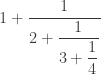
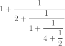
Hurray! A final answer. The continued fraction reduces to . But what if we tried to go the other way? Suppose we started with a different fraction like , how could we find the continued fraction?

First, treat the fraction like a division problem, , then use division to determine the remainder (in this case, the remainder is 11)

Then just repeat the process but this time, use the 31 and the 11 in our division problem :

Repeat again with :

Repeat again with :

Repeat again with :

Finally, we get a zero remainder, and this means we are done. Now we look back at all of the quotients (the first number after the equal sign) and pop them into a continued fraction:

Tada! We have found our continued fraction. Don’t believe me? If you carefully work through all the steps of fraction arithmetic, you will find that this complicated mess of fractions reduces to , our original number. This algorithm has a special name, the Euclidean algorithm. It is named after the ancient Greek mathematician Euclid, who first published the step by step process in 300 BCE.[1]

For practice, try this algorithm out on our first fraction, . We know that the answer should be:

See if you can recreate it using the ancient algorithm. You might be surprised how powerful a dusty old piece of mathematics can be.

---

[1] https://en.wikipedia.org/wiki/Euclidean_algorithm

Divisibility Rules (7 and 11)

In this blog series, I am exploring a few of my favourite algorithms in mathematics.

Last week, we looked at an algorithm that allowed us to determine if a number was divisible by 3 and 9. This week, I want to explore divisibility rules for 7 and 11.

For example, is divisible by 7?

Perhaps numbers that are divisible by 7 have a nice pattern, like the numbers that are divisible by 2. If we start at 7, and list all numbers divisible by 7, we get the following list:

And unfortunately, this list is not good news. Notice that these numbers end in every possible digit! This is the same problem we had last week when we investigated the rule for the number 3. This means we need a method, an algorithm, to get us on our way.

First, pop off the last digit, 2. Next we double it, 2 doubled is 4. Finally, we subtract it from what is left of the number:

Then we just repeat this process over and over.

pop, double-subtract

pop, double-subtract

pop, double-subtract

Finally, we have the number 21, which is on our list. Hence, divisible by 7.

Why does this process work? Let’s look at a smaller number, say .

Since 49 is on our list, divisible by 7.

The first step, popping off the 8, is actually subtraction:

The next step, is actually . Although it seemed like we doubled the 8, to keep the place value correct, we actually multiplied the 8 by 20. Doing both steps at once looks like this:

Since the pop step is subtracting 8, and the double-subtract is subtracting 20 groups of 8, we could save time and just subtract 21 groups of 8. This would look like:

And this is the key insight. Since 21 is divisible by 7, subtracting 21 groups of anything won’t change our answer. However, it will make our number smaller and easier to deal with. By performing these 2 steps over and over, our number shrinks to a size where we can recognize whether or not it is a multiple of 7.

Funny enough, this style of algorithm also works for 11. In this case, you only have to subtract it, no doubling required. For the process would look like:

pop, subtract

pop, subtract

pop, subtract

pop, subtract

Unfortunately, 24 is not divisible by 11, so . But, if we drop our original number by 2 and try …

Hurray! Since 22 is divisible by 11, we know must be divisible by 11.

For even more rules, check out the Wikipedia page on divisibility.[1] For example, the rule for 13 involves multiplying by 9 before you subtract. Crazy stuff!

---

[1] https://en.wikipedia.org/wiki/Divisibility_rule